The invisible bridge that supports all modern radio
When a radio amateur uses a digital mode, watches a waterfall, listens to an FT8 signal, or transmits a file via VARA, they are unknowingly crossing a fundamental bridge: the one that connects the continuous world of radio waves to the discrete world of numbers. It is a silent, almost invisible transition, but it is the foundation of everything we today call “digital radio.”
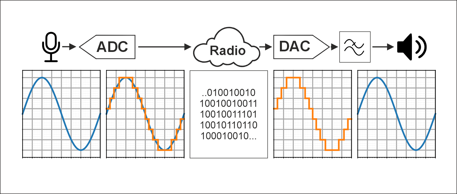
A radio signal, by its very nature, is an analog phenomenon: a wave that varies continuously over time. A computer, instead, lives in a universe made of discrete values, samples, and numbers. Analog-to-digital conversion is the process that allows these two worlds to communicate. It is what enables software to “see” a radio signal and, at the same time, to generate a waveform that a transceiver can transmit into the air.
It is a process that happens tens of thousands of times per second, automatically, yet without it none of the modern digital modes would exist.
From continuous to discrete: how a digital signal is born
To understand analog-to-digital conversion, we must start from a seemingly simple idea: measuring the instantaneous value of a signal at regular time intervals. Each individual measurement is called a sample, and each sample is represented as a number. It is a bit like photographing a moving wave: the more frames you capture per unit of time, the more faithfully you can reconstruct the original motion.
This process is divided into four distinct stages, which are worth exploring one by one.
Sampling
Sampling is the act of “photographing” the analog signal at precise and regularly spaced time instants. The rate at which these measurements are taken is called the sampling frequency (or sample rate) and is measured in samples per second, i.e., Hertz. A 48 kHz sampling rate, common in modern sound cards, means the signal is measured 48,000 times every second.
Here a fundamental principle of digital electronics comes into play, known as the Nyquist–Shannon theorem: to faithfully reconstruct a signal, the sampling frequency must be at least twice the highest frequency present in the signal. In other words, if you want to correctly capture components up to 3 kHz — the typical voice bandwidth in SSB radio — you must sample at at least 6 kHz. Audio interfaces used in amateur radio typically operate at 8, 44.1, or 48 kHz, comfortably covering the relevant audio range.
If you attempt to sample a signal containing frequencies higher than half the sampling rate, an unwanted phenomenon called aliasing occurs: high-frequency components are “folded” into lower frequencies, generating artifacts that do not exist in the original signal. To prevent this, an analog anti-aliasing low-pass filter is placed before the ADC to remove frequencies above the Nyquist limit.
Quantization
Once the sample is obtained, its value — which in nature can take infinitely many values within a continuous range — must be converted into an integer number. This process is called quantization. The ADC divides the signal’s voltage range into a finite number of discrete levels and assigns each sample the nearest level to the measured value.
The number of available levels depends on the bit resolution of the converter. With 8 bits there are 256 distinct levels; with 16 bits there are 65,536; with 24 bits there are over 16 million. Each additional bit doubles the number of levels and theoretically improves the signal-to-noise ratio by about 6 dB. Modern sound cards used in amateur radio typically operate at 16 or 24 bits, with performance more than sufficient for current digital modes.
The difference between the true sample value and the quantized value is called the quantization error, which appears as low-level noise spread across the spectrum. With sufficient resolution, this noise becomes negligible.
Data transmission
Once the signal has been sampled and quantized, the resulting numerical data are transferred to the processor or software through standardized digital interfaces. Consumer sound cards typically use USB or PCI-E interfaces; modern transceivers often adopt protocols such as I²S (Inter-IC Sound) or S/PDIF. The data flow as continuous bitstreams synchronized with the sampling rate. In the amateur radio context, this digital stream is delivered to SDR software or a digital mode decoder, which processes it in real time.
The reverse path: from numbers back to waves
The digital-to-analog conversion (DAC) performs the inverse operation: it takes a sequence of numbers — generated by digital mode software, a voice codec, or an SDR modulator — and turns it into a continuous electrical signal. This process also occurs in multiple stages.
Waveform reconstruction
The DAC receives the numerical samples and, for each one, produces a corresponding voltage level, held constant for the duration of one sampling interval. The immediate result is a staircase-like waveform: technically called a zero-order hold signal. Although it already contains all the information of the original signal, this waveform includes unwanted high-frequency components generated by its discontinuous nature.
The output low-pass filter
To remove these spurious components and obtain a smooth continuous wave, the DAC output is passed through an analog low-pass filter, called a reconstruction filter or interpolation filter. This filter — often active in modern systems, implemented with operational amplifiers or Sallen-Key topologies — removes all components above the Nyquist frequency (half the sampling rate), allowing only the useful frequencies to pass. The result is a faithful analog signal, with a smooth waveform ready to be fed into the microphone or line input of the transceiver.
The quality of this filter is important: a non-flat frequency response or nonlinear phase can introduce subtle distortions that degrade the signal modulation. In high-end transceivers, this stage is carefully engineered.
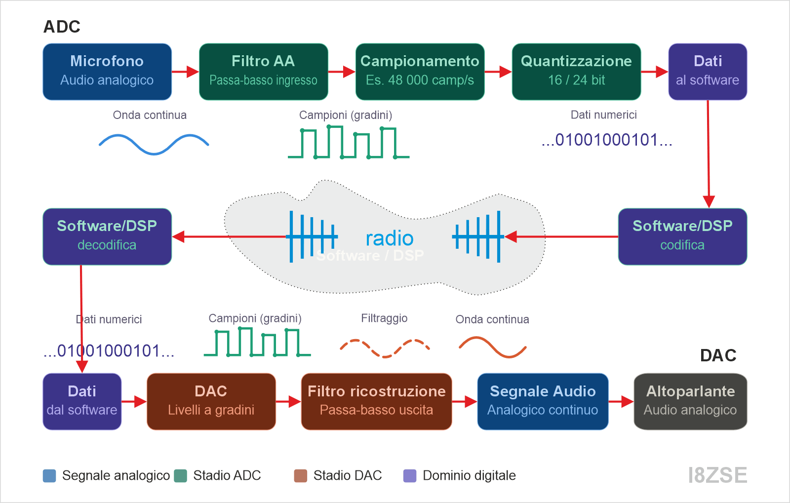
The diagram above illustrates the full path: in the top row the ADC path (from analog reception to digital data), in the bottom row the DAC path (from numerical data back to the transmitted signal). By clicking each block it is possible to explore each stage in detail.
When dedicated modems were required
Those who lived through the pioneering years of digital modes will remember that analog-to-digital conversion was far from trivial. Computers lacked the power and interfaces to directly handle radio signals. Dedicated modems were required, such as TNCs (Terminal Node Controllers), hardware interfaces that handled all modulation and demodulation instead of the computer. The modem was the real protagonist: it generated AFSK tones, decoded signals, and managed the AX.25 protocol. The computer merely sent and received ready-made packets. It was a world where hardware did the heavy lifting and software acted as a simple coordinator. Today this seems distant, but it was the first step toward modern digital radio.
The modem becomes software
With the arrival of inexpensive and powerful sound cards, and the diffusion of DSP capabilities in PCs, the modem became software. It was a silent but complete revolution. Today almost all amateur digital modes — FT8, JS8Call, PSK31, Olivia, RTTY, VARA, FreeDV — simply use the computer’s audio interface. The sound card samples the received signal, converts it into numbers, and delivers it to software. In the same way, it generates tones for transmission and sends them to the radio. The modem is no longer an external box: it is an algorithm, a mathematical function, a piece of code. This has made digital modes more accessible, cheaper, and far more flexible. Changing software means changing mode. This is one of the reasons digital modes have exploded over the last twenty years.
Codecs: digital voice and compression
When moving from data transmission to digital voice, another fundamental element comes into play: the codec. A codec is an algorithm that compresses and reconstructs voice, turning it into a much more compact bitstream than uncompressed audio would require. Without codecs, digital voice over radio would be practically impossible: even at 8 kHz sampling and 16-bit resolution, uncompressed audio would require about 128 kbit/s, far beyond the capacity of any narrowband radio channel. Systems such as D-STAR (using AMBE+2), DMR (AMBE+2 or AMBE++), C4FM/System Fusion (AMBE-3000), and FreeDV (Codec2, open source) use different codecs, each with different philosophies and performance characteristics. This is a complex and fascinating topic that deserves a dedicated chapter, because it directly affects voice quality, signal robustness, and interoperability between devices. Here it is enough to remember that digital voice means sampled, compressed, encoded, and numerically reconstructed speech.
The detail that makes the difference: audio levels
If analog-to-digital conversion is the bridge between radio and computer, audio levels are the bolts that hold that bridge together. Incorrect adjustment can completely compromise the quality of a digital signal. Excessively high levels lead to clipping in the converter: the waveform is truncated at the peaks, introducing harmonic distortion that pollutes the spectrum and makes decoding difficult. Too-low levels, on the other hand, result in insufficient signal-to-noise ratio: only a small portion of the converter’s resolution is used, increasing quantization error.
Every radio amateur using digital modes quickly learns that level adjustment is an integral part of the mode itself. It must be done carefully, observing the waterfall, the transceiver’s ALC meter, and the software level indicators. The general rule is to keep the audio signal around 50–70% of full scale, with peaks that never reach saturation. A good analog-to-digital conversion always starts with correct audio levels: a simple gesture, but the key to a clean and decodable signal.
Why all this matters today
Analog-to-digital conversion is the foundation of everything we call “digital” in amateur radio. It enables WSJT-X software to decode signals at the noise floor, SDR receivers to turn a computer into a full analysis tool, digital voice systems to compress and transmit narrowband speech, wideband links to use complex modulations such as QAM or OFDM, and modern transceivers to integrate advanced DSP functions directly into firmware.
It is an invisible but omnipresent technology, which has transformed the way radio is done just as much as the earlier transition from vacuum tubes to transistors did.
In summary
Analog-to-digital conversion is the heart of modern digital modes. The analog radio signal is sampled at regular intervals (at least twice the highest useful frequency, according to the Nyquist–Shannon theorem), quantized into a finite number of levels (typically 16 or 24 bits), transmitted as a data stream to software, and finally reconstructed by the DAC through a low-pass filter that removes spurious components and restores a continuous waveform. Once required dedicated hardware modems; today a sound card is enough. Codecs compress digital voice down to just a few kilobits per second, and correct audio level adjustment is essential to fully exploit converter resolution and avoid distortion.
For a radio amateur who truly wants to understand how digital modes work, this is one of the most important chapters: it is where the analog world of radio meets the digital world of computing, and where today’s radio is born.